这篇论文一作为陈天齐，XGBoost是从竞赛pk中脱颖而出的算法，目前开源在github，和传统gbdt方式不同，XGBoost对loss function进行了二阶的泰勒展开，并增加了正则项，用于权衡目标函数的下降和模型的复杂度[12]。罗列下优势：

1. 可扩展性强
2. 为稀疏数据设计的决策树训练方法
3. 理论上得到验证的加权分位数略图法
4. 并行和分布式计算
5. 设计高效核外计算，进行cache-aware数据块处理

分布式训练树模型boosting方法已有[1,2,3]。

整体目标

其中$L\left( \cdot \right)$为目标函数，$l(\cdot)$是损失函数，通常是凸函数，用于 刻画预测值${{{\hat y}_i}}$和真实值${{y_i}}$的差异，第二项$\Omega \left( \cdot \right)$为模型的正则化项， 用于降低模型的复杂度，减轻过拟合问题，类似的正则化方法可以在引文[4]看到。模型目标是最小化目标函数。
$L\left( \cdot \right)$为函数空间上的表达，我们可以将其转换为下面这张gradient boosting的方式，记${\hat y}^{(t)}_i$为第$i$个样本第$t$轮迭代：
$${L^{\left( t \right)}} = \sum\limits_{i = 1}^n {l\left( {{y_i},{{\hat y}_i}^{\left( {t - 1} \right)} + {f_t}\left( {{{\bf{x}}_i}} \right)} \right)} + \Omega \left( {{f_t}} \right)$$
对该函数在${\hat y}^{(t)}_i$位置进行二阶泰勒展开，可以加速优化过程，我们得到目标函数的近似：
$${L^{\left( t \right)}} \simeq \sum\limits_{i = 1}^n {\left[ {l\left( {{y_i},{{\hat y}^{\left( {t - 1} \right)}}} \right) + {g_i}{f_t}\left( {{{\bf{x}}_i}} \right) + {1 \over 2}{h_i}f_t^2\left( {{{\bf{x}}_i}} \right)} \right]} + \Omega \left( {{f_t}} \right)$$
泰勒展开的推导部分，可以参考思考1，其中第一项是常数项，删除可得：
$${{\tilde L}^{\left( t \right)}} = \sum\limits_{i = 1}^n {\left[ {{g_i}{f_t}\left( {{{\bf{x}}_i}} \right) + {1 \over 2}{h_i}f_t^2\left( {{{\bf{x}}_i}} \right)} \right]} + \Omega \left( {{f_t}} \right)--(1)$$
下面对正则化项进行参数化定义。延续前文GBDT的概念，引入分裂节点$j$定义的区域记作 $${I_j} = \left\{ {i|q\left( {{{\bf{x}}_i}} \right) = j} \right\}$$
那么$\Omega$展开原目标函数改写为：
$$\eqalign{ & {{\tilde L}^{\left( t \right)}} = \sum\limits_{i = 1}^n {\left[ {{g_i}{f_t}\left( {{{\bf{x}}_i}} \right) + {1 \over 2}{h_i}f_t^2\left( {{{\bf{x}}_i}} \right)} \right]} + \gamma T + {1 \over 2}\lambda \sum\limits_{j = 1}^T {w_j^2} \cr & \;\;\;\;\;{\rm{ = }}\sum\limits_{j = 1}^T {\left[ {\left( {\sum\limits_{i \in {I_j}} {{g_i}} } \right){w_j} + {1 \over 2}\left( {\sum\limits_{i \in {I_j}} {{h_i}} + \lambda } \right)w_j^2} \right]} + \gamma T \cr} --(2)$$
对于固定的树结构$q(x)$，对$w_j$求导得解析解$w^*_j$:
$$w_j^* = {{\sum\limits_{i \in {I_j}} {{g_i}} } \over {\sum\limits_{i \in {I_j}} {{h_i} + \lambda } }}$$
代入到$(1)$式中，可得
$${{\tilde L}^{\left( t \right)}}\left( q \right) = - {1 \over 2}{{{{\left( {\sum\limits_{i \in {I_j}} {{g_i}} } \right)}^2}} \over {\sum\limits_{i \in {I_j}} {{h_i} + \lambda } }} + \gamma T--(3)$$
公式$(3)$可以作为分裂节点的打分，形式上很像CART树纯度打分的计算，区别在于它是从目标函数中推导而得。图中显示目标函数值的计算：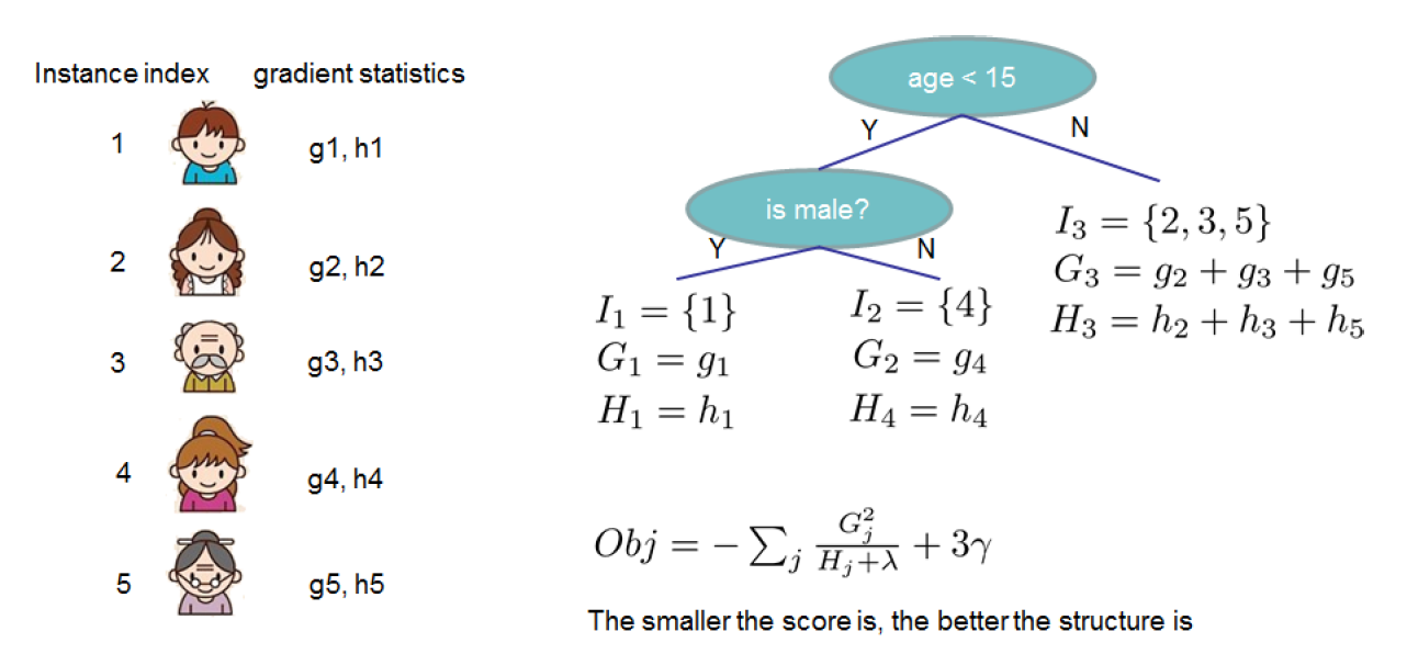

实践中，很难去穷举每一颗树进行打分，再选出最好的。通常采用贪心的方式，逐层选择最佳的分裂节点。假设$I_L$和$I_R$为分裂节点的左右节点，记$I=I_L \cup I_R$。
则选择此节点分裂的收益为：
$${L_{split}} = {1 \over 2}\left[ {{{{{\left( {\sum\limits_{i \in {I_L}} {{g_i}} } \right)}^2}} \over {\sum\limits_{i \in {I_L}} {{h_i} + \lambda } }} + {{{{\left( {\sum\limits_{i \in {I_J}} {{g_i}} } \right)}^2}} \over {\sum\limits_{i \in {I_J}} {{h_i} + \lambda } }} - {{{{\left( {\sum\limits_{i \in I} {{g_i}} } \right)}^2}} \over {\sum\limits_{i \in I} {{h_i} + \lambda } }}} \right] - \gamma \;\;-- (4)$$
[补充]
1.作为GB类方法，也可以采用shrinkage策略
2.随机森林[5]的特征降采样(subsampling)克服过拟合代码，xgboost用了类似的技术。和传统的降采样不同，xgboost按列进行降采样，在并行化有加速作用。(待研究)

查找分裂节点(split finding)

贪心算法
贪心算法是最基本的方法，前面介绍的时候有提过。具体做法：遍历所有特征中可能的分裂点位置，根据公式$(4)$找到最合适的位置。$Split\_Finding()$算法流程如下
$$\eqalign{ & Split\_Finding(): \cr & Input:I,instance\;set\;of\;current\;node \cr & Input:d,feature\;dimension \cr & gain \leftarrow 0 \cr & G \leftarrow \sum\limits_{i \in I} {{g_i}} ,H \leftarrow \sum\limits_{i \in I} {{h_i}} \cr & for\;k = 1\;to\;m\;do \cr & \;\;\;\;{G_L} \leftarrow 0,{H_L} \leftarrow 0 \cr & \;\;\;\;for\;j\;in\;sorted\left( {I,by\;{{\bf{x}}_{jk}}} \right)\;do \cr & \;\;\;\;\;\;\;\;{G_L} \leftarrow {G_L} + {g_j},{H_L} \leftarrow {H_L} + {h_j} \cr & \;\;\;\;\;\;\;\;{G_R} \leftarrow G - {G_L},{H_R} \leftarrow H - {H_L} \cr & \;\;\;\;\;\;\;\;score \leftarrow \max \left( {score,{{G_L^2} \over {{H_L} + \lambda }} + {{G_R^2} \over {{H_R} + \lambda }} - {{{G^2}} \over {H + \lambda }}} \right) \cr & \;\;\;\;end \cr & end \cr & Output:\; split\_value\; with\; max \; score}$$
近似算法
如果数据不能一次读入内存，使用贪心算法效率较低。近似算法在过去也有应用[6, 7, 8]。具体描述为，对于某个特征${\bf x}_k$，找到该特征若干值域分界点$\{s_{k1}, s_{k2}, ... ,s_{kl}\}$。根据特征的值对样本进行分桶，对于每个桶内的样本统计值$G$、$H$进行累加（两个统计量含义同贪心算法），记为分界点$v$的统计量，$v$满足$\{{\bf x}_{kj}=s_{kv}\}$。最后在分界点集合上调用$Split\_Finding()$进行贪心查找，得到的结果为最佳分裂点的近似。具体如下：
$$\eqalign{ & for\;k = 1\;to\;m\;do \cr & \;\;\;\;Propose\;{S_k} = \left\{ {{s_{k1}},{s_{k2}},...,{s_{kl}}} \right\}\;by\;percentile\;on\;feature\;k \cr & \;\;\;\;Propose\;can\;be\;done\;per\;tree\left( {global} \right),or\;per\;split\left( {local} \right) \cr & end \cr & for\;k = 1\;to\;m\;do \cr & \;\;\;\;{G_{kv}} \leftarrow = \sum\limits_{j \in \left\{ {j|{s_{k,v}} \ge {x_{jk}} > {s_{k,v - 1}}} \right\}} {{g_j}} \cr & \;\;\;\;{H_{kv}} \leftarrow = \sum\limits_{j \in \left\{ {j|{s_{k,v}} \ge {x_{jk}} > {s_{k,v - 1}}} \right\}} {{h_j}} \cr & end \cr & call\;Split\_Finding\left( {} \right) \cr}$$
下面介绍找特征值域分界点$\{s_{k1}, s_{k2}, ... ,s_{kl}\}$的方法，加权分位数略图。为了尽可能地逼近最佳分裂点，我们需要保证采样后数据分布同原始数据尽可能一致。记${D_k} = \left\{ {\left( {{x_{1k}},{h_1}} \right),\left( {{x_{2k}},{h_2}} \right) \cdots \left( {{x_{nk}},{h_n}} \right)} \right\}$表示 每个训练样本的第$k$维特征值和对应二阶导数。接下来定义排序函数为$r_k(\cdot):R \rightarrow[0, +\infty)$
$${r_k}\left( z \right) = {1 \over {\sum\limits_{\left( {x,h} \right) \in {D_k}} h }}\sum\limits_{\left( {x,h} \right) \in {D_k},x < z} h$$
函数表示特征的值小于$z$的样本分布占比，其中二阶导数$h$可以视为权重，后面论述。在这个排序函数下，我们找到一组点$\{s_{k1}, s_{k2}, ... ,s_{kl}\}$ ,满足：
$$\left| {{r_k}\left( {{s_{k,j}}} \right) - {r_k}\left( {{s_{k,j + 1}}} \right)} \right| < \varepsilon$$
其中，${s_{k1}} = \mathop {\min }\limits_i {x_{ik}},{s_{kl}} = \mathop {\max }\limits_i {x_{ik}}$。$\varepsilon$为采样率，直观上理解，我们最后会得到$1/\varepsilon$个分界点。
讨论下为何$h_i$表示权重。从目标函数$(1)$出发，配方得到 $$\sum\limits_{i = 1}^n {\left[ {{1 \over 2}{{\left( {{f_t}\left( {{x_i}} \right) - {g_i}/{h_i}} \right)}^2}} \right]} + \Omega \left( {{f_t}} \right) + constant$$
具体证明过程见原作附录。这是一个关于标签为${{g_i}/{h_i}}$和权重为$h_i$的平方误差形式。当每个权重相同的时候，退化为普通的分位数略图[9, 10]
接下来介绍另一个论文的亮点，寻找分裂点的过程中，如何克服数据稀疏。稀疏数据可能来自于missing value、大量的0值、或者特征工程例如采用one-hot表示带来的。为了解决这个问题，设定一个默认指向，当发生特征缺失的时候，将样本分类到默认分支，如下图：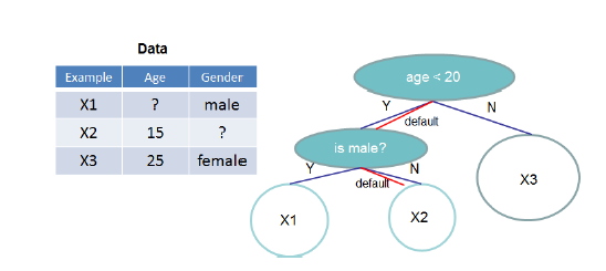

默认方向由训练集中non-missing value学习而得，把不存在的值也当成missing value进行学习和处理，如下：
$$\eqalign{ & Sparsity\_Split\_Finding(): \cr & Input:I,instance\;set\;of\;current\;node \cr & Input:d,feature\;dimension \cr & gain \leftarrow 0 \cr & G \leftarrow \sum\limits_{i \in I} {{g_i}} ,H \leftarrow \sum\limits_{i \in I} {{h_i}} \cr & for\;k = 1\;to\;m\;do \cr & \;\;\;\;{G_L} \leftarrow 0,{H_L} \leftarrow 0 \cr & \;\;\;\;for\;j\;in\;sorted\left( {I_k,ascent order by\;{{\bf{x}}_{jk}}} \right)\;do \cr & \;\;\;\;\;\;\;\;{G_L} \leftarrow {G_L} + {g_j},{H_L} \leftarrow {H_L} + {h_j} \cr & \;\;\;\;\;\;\;\;{G_R} \leftarrow G - {G_L},{H_R} \leftarrow H - {H_L} \cr & \;\;\;\;\;\;\;\;score \leftarrow \max \left( {score,{{G_L^2} \over {{H_L} + \lambda }} + {{G_R^2} \over {{H_R} + \lambda }} - {{{G^2}} \over {H + \lambda }}} \right) \cr & \;\;\;\;end \cr & \;\;\;\;{G_R} \leftarrow 0,{H_R} \leftarrow 0 \cr & \;\;\;\;for\;j\;in\;sorted\left( {I_k,ascent order by\;{{\bf{x}}_{jk}}} \right)\;do \cr & \;\;\;\;\;\;\;\;{G_R} \leftarrow {G_R} + {g_j},{H_R} \leftarrow {H_R} + {h_j} \cr & \;\;\;\;\;\;\;\;{G_L} \leftarrow G - {G_R},{H_L} \leftarrow H - {H_R} \cr & \;\;\;\;\;\;\;\;score \leftarrow \max \left( {score,{{G_L^2} \over {{H_L} + \lambda }} + {{G_R^2} \over {{H_R} + \lambda }} - {{{G^2}} \over {H + \lambda }}} \right) \cr & \;\;\;\;end \cr & end \cr & Output:\; split\_value\; and\; default \;directions\; with\; max \; score}$$

论文后续内容为系统部分（包括并行化、cache-aware加速、数据块预处理，需要结合代码研读）、实验（在不同的数据集上进行了实验，包括分类、LTR、CTR预估）详见论文[11]
代码阅读：
代码易用，注释较完备，支持多种语言，目前仍在持续集成和更新，其中稀疏矩阵存储为CSR格式(见附录思考[2])。
很多核心的机器学习函数复用了作者的另一个机器学习库DMLC(Distributed Machine Learning Common Codebase)，和参考[12]中介绍代码版本对比，运用较多通用的工厂类方法(见附录思考[3])，草草介绍下主体代码组成，下一篇会进行详细拆解：

1
2
3
4
5
6
7
8
9
10
11
12
13
14
15
16
17
18
19
20
21

Data.h 定义基础数据结构，
    如数据信息MetaInfo，稀疏矩阵RowBatch，数据集合RowSet，训练时矩阵表达DMatrix。
Tree_model.h 定义了树相关参数TreeParam，树的模板类TreeModel(对应树节点Node)，
    回归树RegTree，关于树的操作（增删改查，读写load,save,dump2text等）。
Tree_updater.h 完成对树的更新，包含对象工厂类用于注册不同的更新操作:
"updater_colmaker.cc",  通过数据列(论文介绍方式)树的更新（单机多线程版本）
"updater_skmaker.cc",  分位数略图法进行数据采样
"updater_refresh.cc",  更新操作
"updater_prune.cc",  更新过程中进行剪枝
"updater_histmaker.cc",  通过直方图相关统计量完成树的更新
"updater_sync.cc", 从分布训练机器节点中进行树的同步
Objective.h 定义了目标函数，具体优化目标实现，回归,分类,排序函数由对象工厂生成：
"multiclass_obj.cc", 多分类损失函数("SoftmaxMultiClass","SoftprobMultiClass")
"rank_obj.cc", 排序损失函数，有多种可选(PairwiseRankObj，LambdaRankNDCG，LambdaRankObjMAP)
"regression_obj.cc"，回归损失函数("GammaRegression")
看demo可知，xgboost允许用户自定义损失函数。
metric.h 模型效果评估类，包含elementwise_metric、multiclass_metric、rank_metric三类。
"elementwise_metric.cc": 定义评估函数有(RMSE, MAE, logLoss, Error, PosssionNegLoglik, 
    GammaDeviance, GammaNlogLik)
"multiclass_metric.cc": 定义两种评估指标(SoftmaxMultiClass, SoftprobMultiClass)
"rank_metric.cc": 定义评估指标(AMS, Auc, Precision, NDCG, MAP)

附录

引文
[1] Panda, Biswanath, et al. “PLANET: massively parallel learning of tree ensembles with MapReduce.” Proceedings of the Vldb Endowment 2.2(2009):1426-1437.
[2] Tyree, Stephen, et al. “Parallel boosted regression trees for web search ranking.” International Conference on World Wide Web ACM, 2011:387-396.
[3] Ye, Jerry, et al. “Stochastic gradient boosted distributed decision trees.” ACM Conference on Information and Knowledge Management, CIKM 2009, Hong Kong, China, November 2009:2061-2064.
[4] Johnson, Rie, and Z. Tong. “Learning Nonlinear Functions Using Regularized Greedy Forest.” IEEE Transactions on Pattern Analysis & Machine Intelligence 36.5(2013):942-54.
[5] Friedman, Jerome H., and B. E. Popescu. “Importance Sampled Learning Ensembles.” (2003).
[6] Li, Ping, C. J. C. Burges, and Q. Wu. “McRank: Learning to Rank Using Multiple Classification and Gradient Boosting.” Advances in Neural Information Processing Systems (2007):897-904.
[7] Bekkerman, Ron, M. Bilenko, and J. Langford. “Scaling up machine learning: parallel and distributed approaches.” ACM SIGKDD International Conference Tutorials ACM, 2011:1-1.
[8] Tyree, Stephen, et al. “Parallel boosted regression trees for web search ranking.” International Conference on World Wide Web ACM, 2011:387-396.
[9] Greenwald, Michael. “Space-efficient online computation of quantile summaries.” Acm Sigmod Record 30.2(2001):58–66.
[10] Zhang, Qi, and W. Wang. “A Fast Algorithm for Approximate Quantiles in High Speed Data Streams.” (2007):29-29.
[11]Chen, Tianqi, and C. Guestrin. “XGBoost: A Scalable Tree Boosting System.” (2016).
[12] xgboost导读和实战（百度云地址），王超，陈帅华
[13] xgboost代码参数说明, @zc02051126译
[14]xgboost: 速度快效果好的boosting模型,何通
[15]Introduction to Boosted Trees, 官网

思考
[1].不能直接看明白，手痒推导一把就通顺多了。函数$f(x)$在$x_0$处的二阶展开式为： $$f\left( x \right) = f\left( {{x_0}} \right) + f'\left( {{x_0}} \right)\left( {x - {x_0}} \right) + f''\left( {{x_0}} \right){\left( {x - {x_0}} \right)^2}$$
我们对$l(y_i, x)$在${\hat y}^{(t-1)}_i$处进行二阶展开得到
$$l({y_i},x) = l\left( {{y_i},{{\hat y}^{\left( {t - 1} \right)}}} \right) + {{\partial l\left( {{y_i},{{\hat y}^{\left( {t - 1} \right)}}} \right)} \over {\partial {{\hat y}^{\left( {t - 1} \right)}}}}\left( {x - {{\hat y}^{\left( {t - 1} \right)}}} \right) + {{{\partial ^2}l\left( {{y_i},{{\hat y}^{\left( {t - 1} \right)}}} \right)} \over {\partial {{\hat y}^{\left( {t - 1} \right)}}}}{\left( {x - {{\hat y}^{\left( {t - 1} \right)}}} \right)^2}$$
令$x={\hat y}^{(t-1)}+f_t({\bf x}_i)$，且记一阶导为${g_i} = {{\partial l\left( {{y_i},{{\hat y}^{\left( {t - 1} \right)}}} \right)} \over {\partial {{\hat y}^{\left( {t - 1} \right)}}}}$，二阶导为${h_i} = {{{\partial ^2}l\left( {{y_i},{{\hat y}^{\left( {t - 1} \right)}}} \right)} \over {\partial {{\hat y}^{\left( {t - 1} \right)}}}}$。
我们得到$l(y_i, {\hat y}^{(t-1)}+f_t({\bf x}_i))$的二阶泰勒展开：
$$l\left( {{y_i},{{\hat y}^{\left( {t - 1} \right)}}} \right) + {g_i}{f_t}\left( {{{\bf{x}}_i}} \right) + {1 \over 2}{h_i}f_t^2\left( {{{\bf{x}}_i}} \right)$$
带入目标函数可得：
$${L^{\left( t \right)}} \simeq \sum\limits_{i = 1}^n {\left[ {l\left( {{y_i},{{\hat y}^{\left( {t - 1} \right)}}} \right) + {g_i}{f_t}\left( {{{\bf{x}}_i}} \right) + {1 \over 2}{h_i}f_t^2\left( {{{\bf{x}}_i}} \right)} \right]} + \Omega \left( {{f_t}} \right)$$

[2]：csr格式是什么？类似的格式有什么，它们之间的区别是什么？
参见：稀疏矩阵存储格式总结+存储效率对比:COO,CSR,DIA,ELL,HYB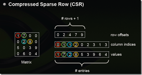

CSR有行偏移，列下标，值三种元素。行偏移数组大小为（总行数目+1），行偏移表示某一行的第一个元素在values里面的起始偏移位置。数值和列号与COO一致，表示一个元素以及其列号。如上图中，第一行元素1是0偏移，第二行元素2是2偏移，第三行元素5是4偏移，第4行元素6是7偏移。在行偏移的最后补上矩阵总的元素个数，本例中是9。

[3]思考：通用的工厂类，@tenfyzhong

ShawnXiao@baidu